Bollinger Mean Reversion Backtest on AAPL: The Dip Buyer Who Never Holds
Mean reversion is the most intuitive idea in trading — buy the dip, sell the bounce. On real daily AAPL data (2018–2025) it returns +19.27% while buy and hold makes +576.91%, and its drawdown is worse than just holding. Python code and charts.
Bollinger Mean Reversion Backtest on AAPL (2018–2025, daily)
Mean reversion is the first strategy a beginner understands and the last one they stop losing money with. "Buy low, sell high" — what could be simpler? I spent my Sunday evenings for a year finding "oversold" stocks, convinced I was being smart while everyone else was just buying. This post is that habit, run properly, on the most famous stock in the world. The results embarrassed me in a useful way. Strategy Lab #11.
The strategy
Bollinger Bands wrap a 20-day moving average with two standard-deviation envelopes:
- Buy when the close falls below the lower band and turns back up inside it.
- Sell when the close returns to the middle band.
29 round trips over 8 years. Notice that: this is a low-turnover strategy, the opposite of the Stochastic crossover I just tested on crypto. On daily AAPL there is no funding cost, no 0.01%/8h drain, and 29 trades pay almost nothing in fees. If this strategy fails, it fails for strategy reasons — not cost reasons. That's a clean experiment.
Results
| Strategy | Category | Total return | CAGR | MaxDD | Sharpe | Trades |
|---|---|---|---|---|---|---|
| bollinger | meanrev | +19.27% | +3.25% | -42.79% | 0.26 | 29 |
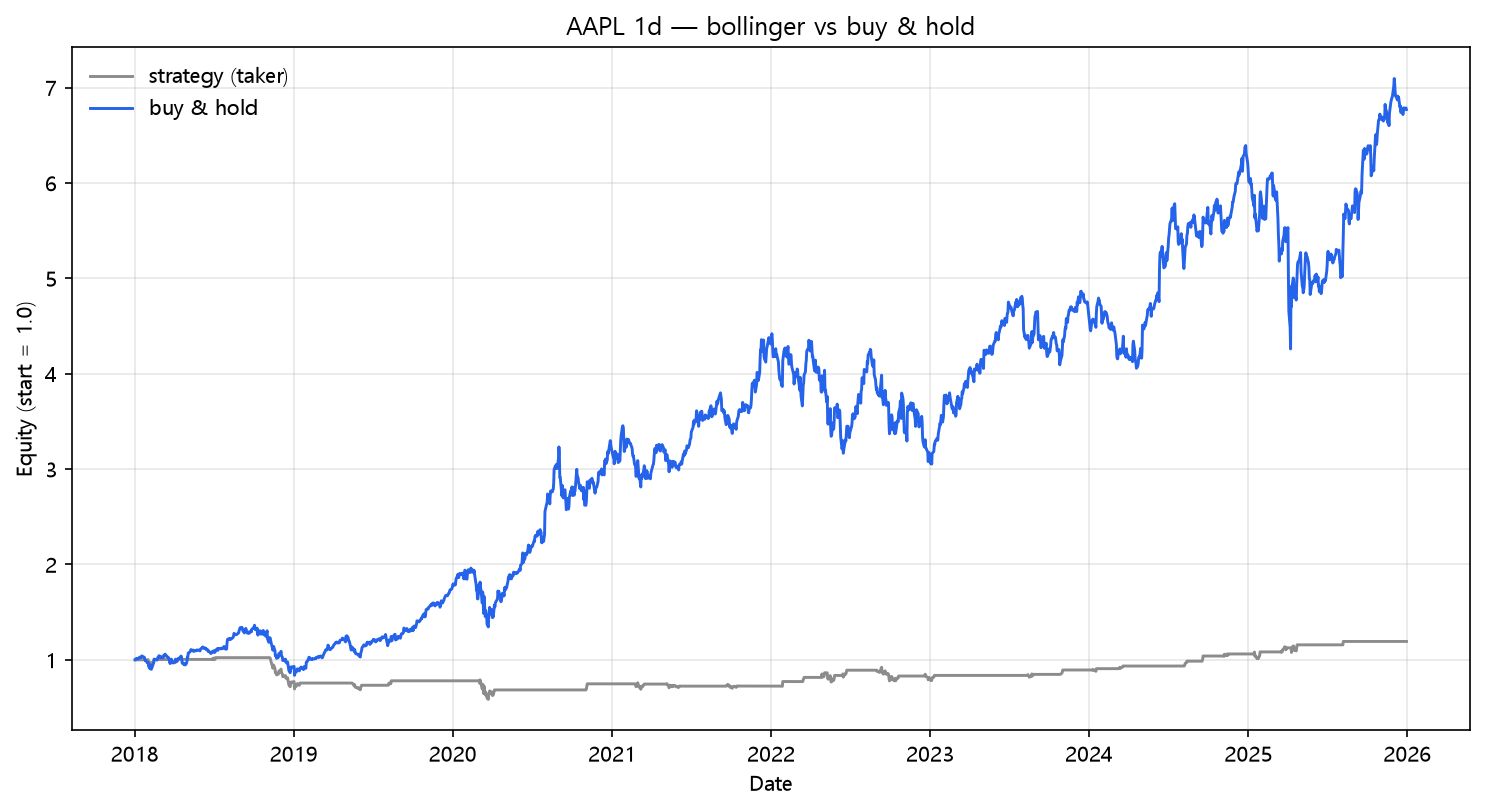
Two numbers tell the whole story:
| Strategy | Total return | CAGR | MaxDD | Sharpe |
|---|---|---|---|---|
| bollinger | +19.27% | +3.25% | -42.79% | 0.26 |
| buy & hold | +576.91% | +41.52% | -38.52% | 1.12 |
AAPL multiplied by 6.8 over the period. Mean reversion captured +19.27% — and suffered a worse drawdown than holding. The strategy's design is the culprit: the exit at the middle band caps every winning trade at "a bounce," so the strategy spent eight years selling the exact thing it should have kept. Meanwhile in 2022, the reversion logic kept buying into the slide — that's where the -42.79% came from, deeper than buy and hold's own 2022 scar.
Fees barely matter here (and that's the point)
| Scenario | Cost/leg | Total return | MaxDD | Sharpe | Trades |
|---|---|---|---|---|---|
| naive (zero cost) | 0.00% | +22.78% | -42.56% | 0.28 | 29 |
| taker fee 0.05%/leg | 0.05% | +19.27% | -42.79% | 0.26 | 29 |
| + funding 0.01%/8h | 0.05% | +19.27% | -42.79% | 0.26 | 29 |
| + slippage 10bp/leg | 0.15% | +12.54% | -43.24% | 0.21 | 29 |
| + slippage 25bp/leg | 0.30% | +3.15% | -43.92% | 0.13 | 29 |
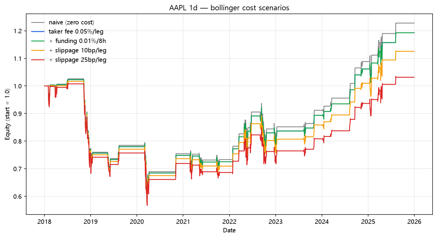
Even with 25bp slippage the return only drops to +3.15% — costs are a rounding error on 29 trades. (The "+funding" row equals the taker row because equities have no funding — that's a crypto-only cost.) Compare this to the crypto hourly posts: the cost model matters inversely with trade count. Low-turnover strategies can be wrong in the strategy itself and you'll never see it in the fee column.
What this does NOT prove
- This is my entry/exit rule (lower-band recovery → middle band). Many Bollinger variants hold to the upper band or add an RSI filter — each is a different strategy with different economics. I'm testing the simplest honest reading.
- One stock, one period. AAPL 2018–2025 is a relentless uptrend, the hardest environment for reversion logic. A rangebound market would favor it more. That's exactly why the cross-market contrast matters: the same strategy is not the same strategy in a different market.
- The robust takeaway isn't "mean reversion is bad." It's: capping your winners at "a bounce" is a conscious choice to never own the trend — and on a stock that quintuples, that choice is expensive.
Code
from backtest_base import fetch, backtest_signal, metrics

df = fetch("AAPL", "yahoo", "2018-01-01", "2025-12-31")   # daily bars
close = df["close"]
mid = close.rolling(20).mean()
lower = mid - 2 * close.rolling(20).std(ddof=0)
enter = ((close > lower) & (close.shift(1) <= lower.shift(1))).fillna(False)
exit_ = (close > mid).fillna(False)

signal = stateful_position(enter, exit_)   # recover above lower band -> mid band
res = backtest_signal(df, signal, cost_per_leg=0.0005, funding_per_bar=0.0)
print(metrics(res, 365))
Reproduce it
cd blog-drafts/scripts
python backtest_base.py --strategy bollinger --source yahoo --symbol AAPL \
    --start 2018-01-01 --end 2025-12-31 --fee 0.0005
Data: yfinance (Yahoo Finance), daily OHLCV, 2,010 bars. The tables above reproduce exactly from this command.
This is a backtest on historical data, not investment advice. Past performance does not predict future results.